1.0 CONTROL ACTIONS
1.1 Two step control action
This can be defined as 'the action of a controller whose output changes from one state to another due to a variation in its input'
One example of this control is that of a float operated filling v/v say for a cistern. In normal condition the output of the float is nil and no water passes through the valve, should the water level drop the float detects this and operates the valve to change to its second state which is open and water flows. When the level re-establishes then the float controls the valve to return to its primary state which is closed. In this way the float is controlling the water level by changing the valve between two different states.
An example commonly found in is shown below
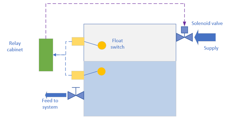
The system works as follows; the level drops until the lower float is uncovered, the controller detects this and opens the filling valve, the filling v/v remains open until the top float is covered and then the controller shuts the valve
The distance between the floats is termed the 'Overlap' i.e. the distance between the high and low controlling values (on some systems this can be altered by altering the high or low set point of the controller, in the above system this would mean altering the position of the floats)
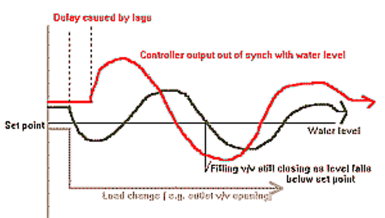
If there were any delays or lags in the sensing side, say the float switch was a little sticky or the filling v/v was slow to fully open then the level would fall below rise above the low and high set points respectively. This is termed 'Overshoot', if the controller 'response to change' time was speeded up so the overshoot could be reduced.
The system may be represented in block form as follows;
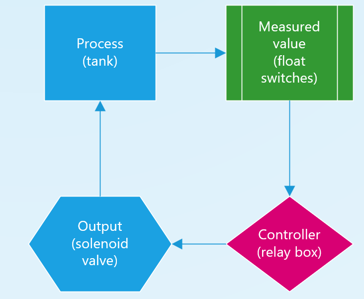
The float switches are the measure values on which the controller (relay box) operates. The signal is being 'fed back' to the controller hence to measured value is Feedback for the controller; i.e. the controller can see the direct results of its action.
Feed forward signals are sometimes used on systems which have an inherently high Process Lag; an example of this may be on a Marine Diesel engine jacket fresh water-cooling system where part of the control is that the inlet temperature to the engine is monitored and fed forward to the controllers, should the temperature at inlet rise then consequently the outlet temperature must also rise. As the rise has already been detected then the controller can start increasing the sea water cooling to the jacket water coolers even though no temperature rise on the outlet from the engine may have been detected. This type of control, as it takes no account of what is happening to the process (is the engine running and hence requires the extra cooling or is it stopped) is not very accurate and normally (and as in this case) required Feedback to improve it. #
1.2 The actions of controllers having variable output
2.0 Proportional control action
The output signal is varied depending on the deviation from the set point. The output signal magnitude is varied by the gain. The greater the gain the greater the output signal magnitude for a given deviation.
This where the change in output signal from a controller is proportional to the change in input signal
The control can be summed up in the following;
Output = Constant x Deviation
Output - this
is the output from the controller and goes to the control element (say the
filling v/v on the previous example i.e. the piece of equipment that actually
alters the process.
Constant- This is the 'Gain' of the
controller, as the output varies with the deviation, the amount it varies can
be altered.
Say if the deviation changes by one unit the output changes by one
unit, hence the gain is one. If the output varied by two for the same one
change in deviation, then the gain would be two. Similarly, if the change in
output was one half a unit for a one unit change in input, then the gain would
be half. Another way used to describe Gain is 'Proportional band', here a gain
of one is described as a proportional band (Pb)of 100%. For a gain of two the
Pb is 50%, and for a gain of a half the Pb is 200%, hence it can be seen that
the magnitude of the Pb is opposite to the gain.
Deviation- This is the difference between
the set point of the controller and the measured value. If the set point was
one unit and the measured value was two units the deviation would be one unit.
Deviation = Set point - Measured value
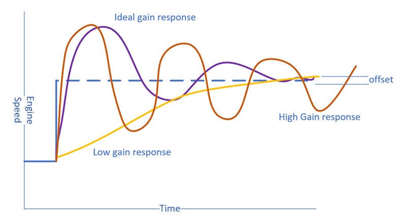
The important thing to remember is that the narrower the Proportional band the higher the gain and hence the higher the output varies for a change in deviation, this has the effect of making the controller control the process quicker by operating the controlling element more for smaller variations measured value. This has the negative effect as will be seen of making the system unstable
2.1 OFFSET
For a proportional controller to work there must be a deviation, if the deviation is zero then the controller output to the controlling element is zero. For the example of the tank and filling v/v obviously this is not possible, with the water constantly flowing out of the manual outlet v/v then the filling valve (or controlling element) must always be some degree open. If the level is at the level of the set point, then the output is nil, the filling v/v is shut and the level drops, deviation occurs and the filling v/v opens. with this it can be seen that the system is not stable; what would happen in reality is the level would change ( say the level was low and was now rising) until it reached a point close to the set point where the deviation multiplied by the gain would give an output signal to the filling v/v such that the flow of water in to the tank equaled the flow of water out of the tank.
This deviation is called 'offset'
Therefore, a proportional only controller
when in equilibrium must have offset
The amount of offset will be determined by the Gain, for the tank system if the
gain is high the deviation can be small for a larger output
The offset will increase for increased loads on the system i.e. if the outlet v/v on the example where to be opened further obviously the filling v/v would have to be opened further, and hence the deviation (offset) to give the required output would have to be greater.
For the system above all the control would be positive as the filling v/v would only be open if the level was low and hence the offset would always be positive, when the level rose above the set point, say caused by Lags leading to Overshoots or the filling v/v leaking slightly the deviation would be negative and the output zero.
2.2 Proportional action and instability (Hunting)
As the gain increases so the output increases for smaller and smaller changes in deviation, eventually the response starts to look similar to that of a two-step controller with the control valve flying from full open to full shut with the slightest deviation from the set point. This would be o.k. if the system was devoid of all Lags, with lags however, particularly between the controller and controlling element, there is a tendency for 'over shoot'.
This can occur with reduced gain when the process lags are increased, for systems with a very large lags even small changes in gain can seriously affect the stability of a system and especially its ability to resist step (or rapid) load changes.
For smaller values of gain the system can be set up to have minimum of hunt and be self-stabilizing .
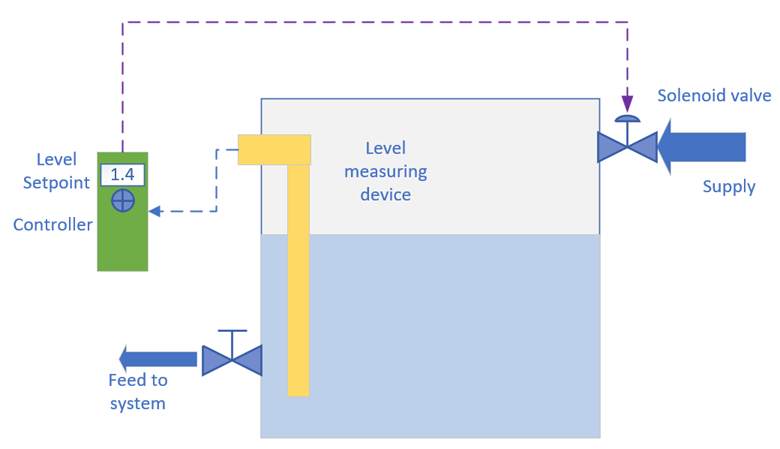
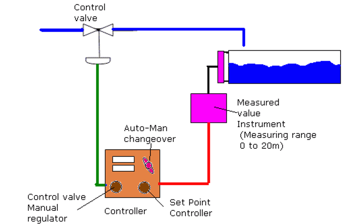
3.0 Split range CONTROL (NEGATIVE and positive offset)
A system could be designed to control both the outlet valves and inlet valves (this is what is seen on the feed water system level control with the spill and filling being controlled from the one controller) ; here the controller would be set up so that when the level is at the set point its output is mid-range ( say for a controller operating in the 3 to 15 psi range this would be 9 psi)
The control valves would be set up so that one, say the filling v/v would go from close at 9.5 psi to open at 15 psi, and the spill v/v would go from close at 8.5 psi to open at 3 psi. The 1 psi in the middle is called the 'Deadband' and is there to ensure both v/vs are not open at the same time. (The v/v acting to open with increasing input signal is called 'Direct Acting' and the v/v closing with increasing pressure is called 'Reverse Acting')
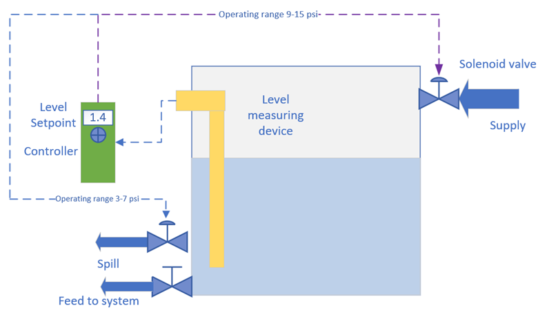
It can be seen that there can now be an offset in the positive i.e. water being used and hence the make-up v/v has to be open and in the negative i.e. there is too much water entering the system and the spill v/v's have to be opened.
Offset is not a desired result of the control of a system, however for proportional only controllers this is a direct consequence. That is why for all controllers performing important functions; including the make-up/spill system controller above other types of controlling action are added to remove the offset
4.0 Integral action (AND the removal of OFFSET)
Integral action is defined as the action of a controller whose output signal changes at a rate proportional to the input (deviation from the set point) signal.
What this means is that if a controller has
a constant deviation, then the integral action controller will increase its
output continuously until it reaches maximum (often referred to as 'Saturation')
If the deviation is zero the integral action controller is zero
If the deviation is small the rate the controller output increases by is small
If the deviation is great then the integral action controller will rapidly
increase its output.
Integral action is included in proportional controllers to remove the inherent offset of the proportional action; the offset is the deviation the integral action requires to alter the output
4.1 Integral action time
The amount of integral action, or how fast the integral action increases or
decreases the output for one unit of deviation is expressed as the time taken
to repeat the proportional action after a stepped change in input.
Rate of increase of output = Deviation x Integral action time
What this means is say the load changes in the simple filling system example by the manual v/v being opened and the level suddenly dropping by a foot, the proportional action will see this load change and give a stepped change in output i.e. if the foot drop in water level equals a change in input signal to the controller of one unit away from the set point, the controller will give a stepped change in output equating to the gain (which is say two ) times the deviation ( one unit) which equals a change in output of two units.
Whilst all this has been going on the integral part of the controller has seen the deviation and has decided to increase the rate of output by an amount equal to the deviation multiplied by the integral action time. The time taken for the output to increase by a further two units (remembering that this was how much the proportional action changed the output) is the integral action time and is measured in seconds.
The shorter the integral action time (less seconds) the more rapidly the integral part of the controller will increase the output; The longer the integral action time the slower the integral action will increase the output.
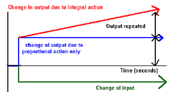
A common way of expressing integral action is in 'Repeats per minute', integral action time is seconds per repeat, hence if the IAT is 10 (seconds per repeat), this would equate to 10/60 minutes per repeat, or more simply 1/6 mins. The repeats per minute is therefore 6.
4.2 Integral action and stability
The introduction of integral action into a controller introduces an extra time lag, remembering the diagram showing that the integral action will take time to increase the output to a stepped load change, whereas the proportional action will give a stepped change. Lags introduce instability, hence it would more difficult to find settings which give a stable output.
Integral action is always used with proportional action
5.0 Derivative action
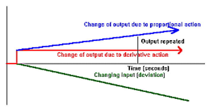
The definition of this is the action of a controller whose output is proportional to the rate of change of input.
That is to say for the filling system if the level was falling slowly the output of the controller would be small. If the level was flying down at a great rate of knots, then the derivative controller would give a high output. It is quite obvious that the derivative action takes no account of the deviation from the set point but is only interested in the rate of change of deviation and hence;
Derivative action by itself cannot be used for control.
The purpose of adding derivative action to a controller is to increase the responses that deviation is removes as quickly as possible. That is to say if the level in our filling system is falling the proportional action will increase the filling at the same rate, however as with seen, if there is a lag in the system particularly between the controller and controlling element; then there is a possibility of instability and a hunt.
If we were at the point where the water level was just starting to fall less rapidly but not at the point where it was actually starting to rise, all the proportional and integral action see is a large deviation and so keep the water v/v wide open, the derivative action, however, sees this slowing down of the drop in water level, its output is dependent on the rate of change and hence reduces, and so the output from the controller reduces.
The introduction of derivative action introduces a stabilizing effect into a control system
5.1 Derivative action time
Output = Derivative action x rate of change of input
Derivative action [coefficient]- This is described as the time the proportional action takes to repeat the derivative action after a ramped (or constant rate of change) input. The units are seconds.
6.0 PID tuning
The setting up of PID controllers is complex and contains many variables. Following are two examples of methods that may be adopted
6.1 Ziegler-Nichols Closed Loop (Hunt) Method
- Set up the system in closed loop i.e. with the controller in auto mode
- Remove integral and derivative action
- Increase the gain (reduce proportional band) until the controller just begins a steady hunt
- record the Proportional Band setting as value P
- Record the periodic time of the sinusoidal hunt as value T
- For Proportional only- Proportional Band = 2 x P
- For Proportional + integral- Proportional band = 2.2 x P, Integral Action Time = T/2
- For Proportional + Integral + Derivative- Proportional band = 1.67 x P, Integral Action Time = T/2, Derivative action time = T/8
6.2 Ziegler-Nichols Open Loop Method
Switch controller to manual ensuring that the system is open loop. i.e. that the controller is disconnected from the controlling unit which can be manually adjusted
Rapidly alter manual regulator to cause a
stepped change in the control valve by a set amount. Record the movement of the
control valve as a percentage of total travel. Record this as δR
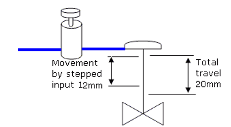
In the above example the valve has moved by 12 out of a total 20mm therefore is
has move 60% of its total travel. δR = 60
Record the system open loop response. That is record the initial valve from the measured valve transmitter, initiate the stepped input then record how the measure valve responds in relation to this
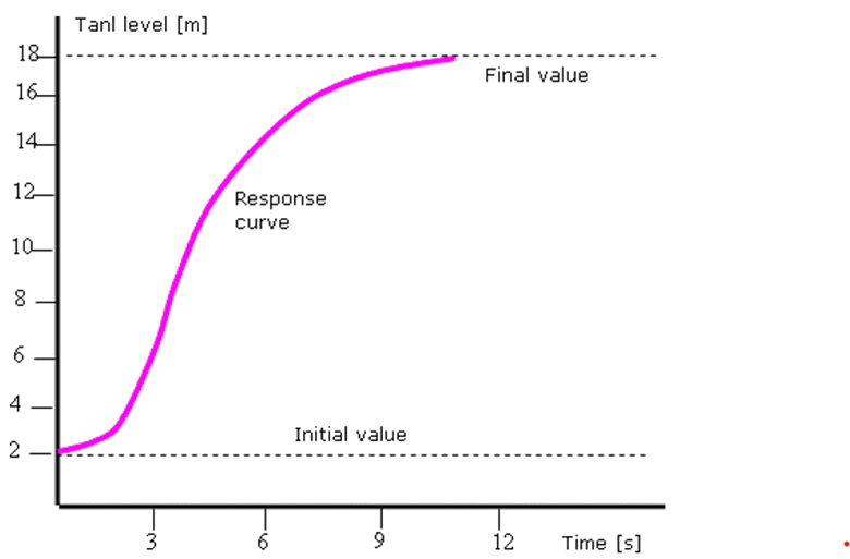
Change the vertical axis of the response graph so that it is scaled as a percentage of the measure value range (which from above we see is 20m).
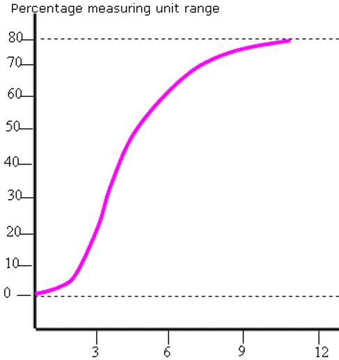
From the graph determine values as best as
possible for dv (distance-velocity- time between controller output signal being
generated and controlled element receiving it) lag T[s]and the maximum slope
N[%/s]
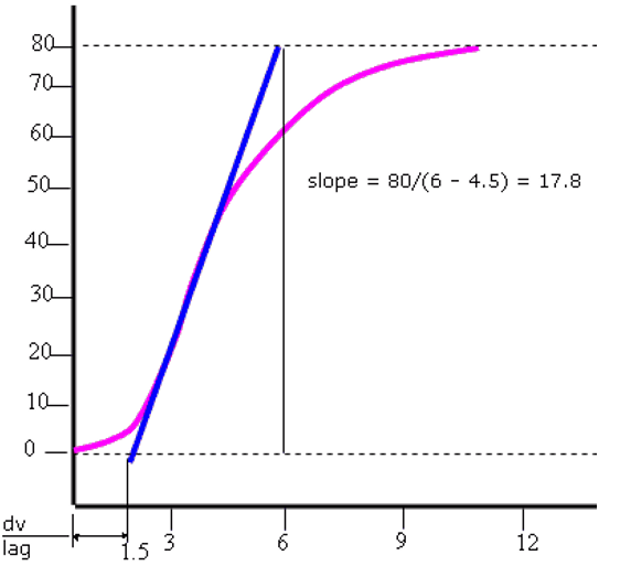
For Proportional only- Proportional Band = N xT/δR x 100%
For Proportional + integral- Proportional band = N x T/δR x 110%, Integral Action Time = 3.33 x T
For Proportional + Integral + Derivative- Proportional band = N x T/δR x 83%, Integral Action Time = 2 x T, Derivative action time = 0.5 x T
For the above worked example this would
give the following results
Proportional only
PB = N x T/δR * 100 = 17.8 x 1.5 / 60 * 100 = 44.5%
Proportional + Integral Action
PB = N x T/δR * 110 = 17.8 x 1.5 / 60 * 110 = 49%
IAT = 3.33 x T = 3.33 x 1.5 = 5 [s]
Proportional + Integral Action +
Derivative Action
PB = N x T/δR * 83 = 17.8 x 1.5 / 60 * 83 = 37%
IAT = 2 x T = 2 x 1.5 = 3 [s]
DAT = 0.5 x T = o.5 * 1.5 = 0.75 [s]
6.3 System responses
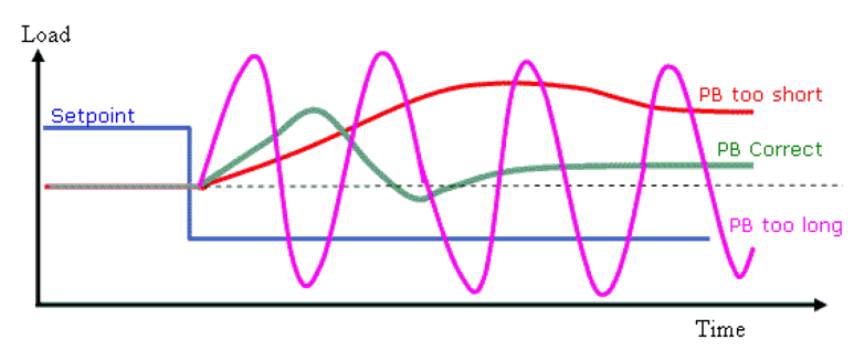
6.3.1 Effects of changing Proportional Band on P controller
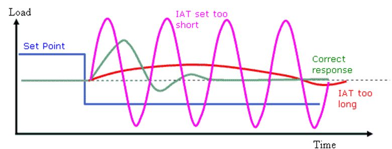
6.3.2 Effects of changing Integral Action Time on P + I controller
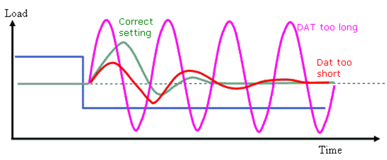
6.3.3 Effects of changing Derivative Action Time on P + I + D controller
7.0 Diaphragm operated control valve
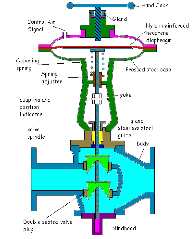
7.1 Hand jack
May be used either for local manual control in the event of signal failure. Or it may be used to prevent or limit opening of the valve
7.2 Valve glands
For accurate valve positioning it is important to keep friction to a minimum. The largest source of friction is the valve gland. For steam valves using asbestos type packing a suitable lubricant must be applied. A better solution takes to form of a pack of several v seals made from Teflon. Fins may be cast or machined into the gland housing for cooling
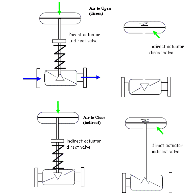
7.3 Fail safe- air to open/close
The control valve may be so designed to fail in either a full open or full closed direction. In addition, the pneumatic signal may open or close the valve
8.0 Appendix: Valve Characteristics
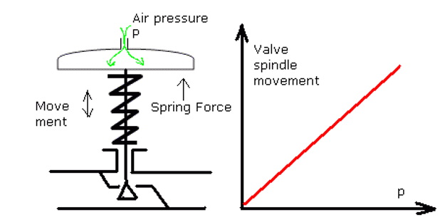
8.1 Pneumatic Valve Characteristic
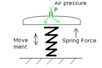
The force acting to compress the spring is given by pressure P x Area A
The force acting against this is given by the spring Constant K x Spring compression distance L
PA = KL
L = P(A/K)
Since the area of the diaphragm and the spring constant are constants for any given set up it can be seen that the spring movement is directly proportional to applied pressure
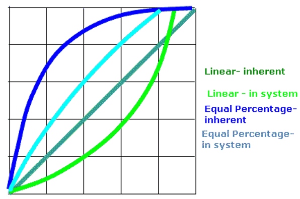
8.2 Inherent or designed characteristic
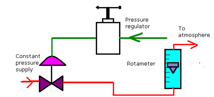
The characteristic of a valve is its relationship between valve lift and flow across it for a constant pressure drop across it. A typical set up for measuring this is shown below
8.3 Quick Opening (poppet) Characteristic
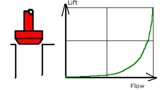
These valves re used in control systems mainly as isolating valves. Their main use is for relief or safety valves. Full bore is achieved at one quarter of the diameter
8.4 Linear Characteristics
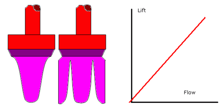
In this design the flow through the valve is proportional to the lift. The normal design is the vee port (or fluted) type although for smaller sizes the plug type is used
#
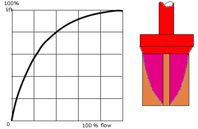
8.5 Equal Percentage Characteristics
In this design for equal increments of valve movement the flow increases by and equal percentage. if the valve is 10mm open and the flow 20, if the valve opens anouther 10mm (100%) the flow increases to 40. If the valve opens a further 10mm (50%) then the flow increases by 50% of 40 which is anouther 20. The action may be expressed as
L = logeQ / K
It should be noted that for true equal percentage the minimum flow is 1%. Therefore, if closing is required some adaption is required
8.6 System characteristics
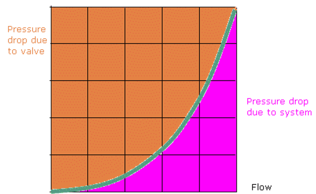
The above graph shows the effects the system has on the flow through the valve. It can be seen that as flow increases the pressure drop across the valve falls thus significantly effecting the characteristic effect of the valve
Fitting a valve with equal percentage trim produces a near linear characteristic. This will be affected by things like varying system pressure drop and maximum flow rates. If the pressure drops across the system is low at the required flow rate, then the pressure drops across the valve will not significantly alter and a linear characteristic should be used.
In practice characteristics are available which offer a balance between linear and equal percentage (parabolic).
9.0 Appendix: Valve Sizing Coefficients
In order to make the purchasing of valves
simple sets of standard valve sizing’s are available. Finding the correct size
may be achieved by use of valve sizing equations.
Calculation must be at the extremes of low and pressure drop and it is standard
practice to oversize to the next size up. Following is a list of the more
common coefficients
9.1 BS4740 Valve Sizing Coefficient Av
Q= Av. √ (ΔP / Ρ)
Q = Flow (usually max rate through valve (m3
/ s)
ΔP = Corresponding Pressure drop across valve (N / m2)
Ρ = Density of liquid (Kg / m3
Av Valve Sizing Coefficient [m2
Due to its units the valve sizing coefficient is often called the Area Coefficient
9.2 American Valve Sizing Coefficient Cv
Q= Cv. √ (ΔP / SG)
Q = Flow (usually max rate through valve
(US Gallons / min)
ΔP = Corresponding Pressure drop across valve (lbft / in2)
SG = Specific (relative) gravity of the liquid relative to water at 20'C
This is the most common coefficient quoted although difficulty in working with the units means it is easier to work in anouther and convert to it
9.3 European Valve Sizing Coefficient Kv
Q= Kv. √ (ΔP / Ρrel)
Q = Flow (usually max rate through valve (m3
/ Hr)
ΔP = Corresponding Pressure drop across valve (Kgf / cm2)
Ρrel = Relative Density of liquid
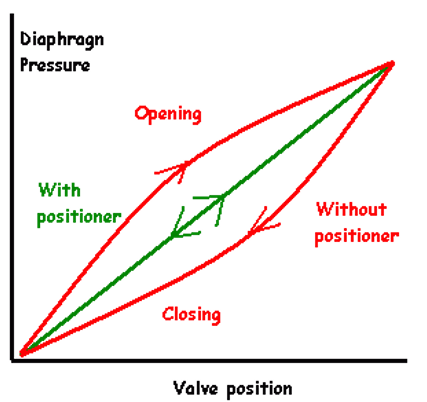
10.0 Valve Positioners
Valve positioners are used on controlling valves where accurate and rapid control is required without error or hysteresis.
- Precise positioning
- can cope with large variations in forces acting on plug
- Rapid positioning
- Removes stiction and friction effects of gland
- Removes effects of large distances between vale and positioner
- Eliminates hysteresis
10.1 Type
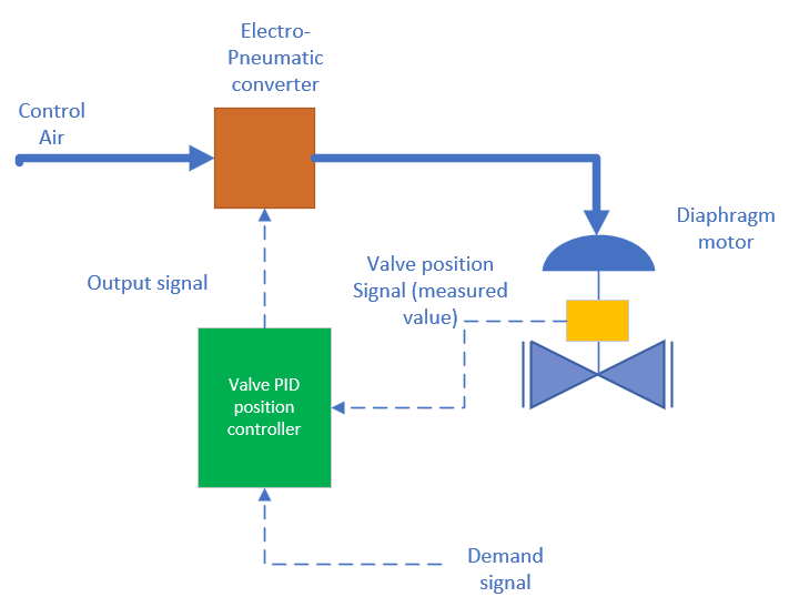
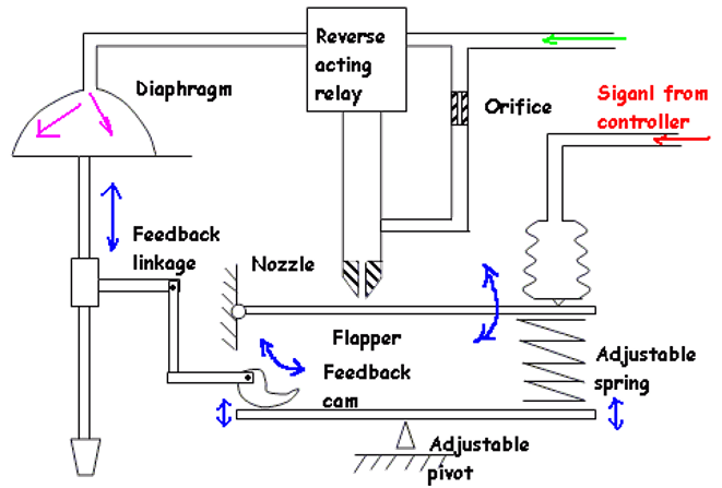
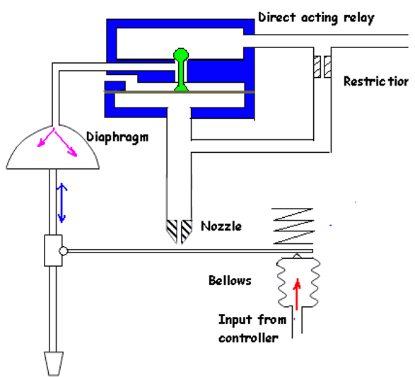
A valve positioner consists of a very high gain amplifier- this may be pneumatic, electric-pneumatic etc, and a feedback link which detects the actual position of the valve.
10.2 Electro-pneumatic
10.3 Pneumatic
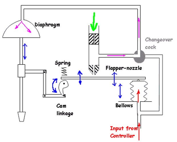
The required movement is for the valve to close. The input pressure from the controller to the bellows falls. The flapper moves away from the nozzle and the pressure after the orifice falls. The pressure to the diaphragm falls and the valve begins to close. The feedback arm moves up rotating the cam clockwise. This raises the beam increasing back pressure in the nozzle until equilibrium is again achieved.
The change over cock allows the signal from the controller to be placed directly on the diaphragm
10.3.1 Force balanced Valve Positioner
10.3.2 Motion balanced Valve Positioner
11.0 Appendix: Torsion meters (shaft power meter)
Torsion meters are used for the measurement of power transferred through a propulsion shaft.
11.1 Principle
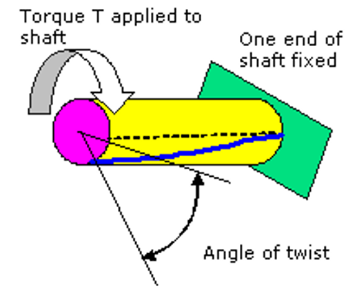
A torque of value T is applied to a shaft of fixed length L and radius r. An
angle of twist θ is generated and is dependent of the modulus of torsional
rigidity G and given by
T/r = Gθ/L
The modulus of rigidity, the radius and the length of the shaft are all fixed thus the torque on the shaft is proportional to the angle of twist
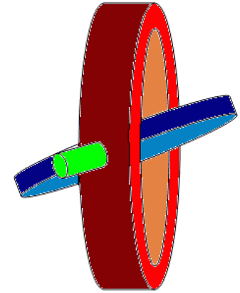
11.2 Typical system
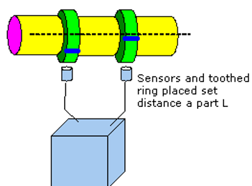
Two AC generators are mounted so that they are driven by the main shaft and
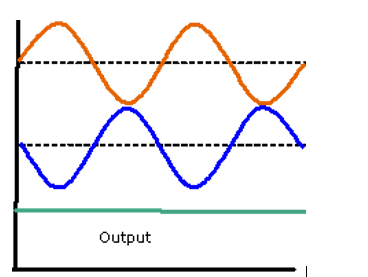
area at set distance apart L. A sinusoidal waveform is produced. One of the
generators is adjusted so that at minimum torque the generated waveforms are
180' out of phase. The outputs from the two generators are then added and the
resultant voltage is used as the measurement of torque
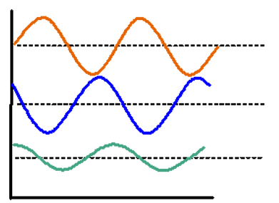
As the torque is applied to the shaft so the twist causes the waveforms to
shift in phase. When the two waveforms are now added an output ac current is
produced which may be amplified and rectified to give an output voltage
proportional to the torque applied to the shaft.
Another method of achieving this is to replace the generators wit sensors and toothed ring.
11.3 Power Calculation
Power is a product of the Torque and revs of the shaft, one of the generator outputs is used to measure the shaft rev/s and a calculation performed
11.4 Magnetic Stress Sensitivity
This type measures magnetic fields in the shaft surface, the distortion of these fields gives an indication of the torque. The principle behind this is that in some ferromagnetic materials reluctance (magnetic resistance) is less along the plane of stress than across it.
In the torductor three rings are fitted around the shaft each ring having four electromagnetic poles. The center ring acts as a transformer primary with the two outer secondary rings having their poles arranged 45' apart to the primary poles but in line with each other. The poles are held in a frame so that there is no contact between the poles and the shaft which have a gap of about 3 mm between them.
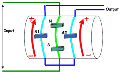
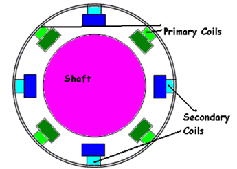
An alternating current is fed to the center ring thus generating a magnetic field. This induces an emf in the outer two rings. The outer two ring coils are connected in series in such a way that at zero stress the emf generated in each ring is opposite and equal in value giving an output of zero volts.
When torque is applied to the shaft the stress lines are distorted axially. The distortion of this field affects the emf induced in the coils increasing on one side and reducing on the other. Thus, a resultant emf of a few millivolts is available at the output. The size of the output is proportional to the stress applied.
12.0 Appendix: Butterfly valve
Consists of a short cylinder generally rubber lined both for corrosion protection and to act as a seal for the disc. The disc forms the closing device and is locked to a spindle. The spindle gland generally takes the form of an O-ring or v-seals.
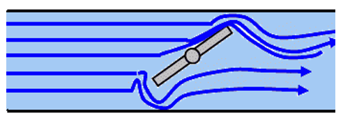
The torque acting on this disc is caused by the dynamics of fluid flow across it. When the valve is partially open the flow across the top half is much smoother than the bottom. This results in a torque acting on the driving spindle
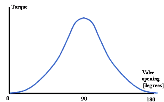
The torque rises from zero to a peak when the valve is in mid position and falls again to zero. This non-linearity makes for difficult accurate positioning. To overcome this, it is normal to fit oversized actuators. The flow through the valve is also very nonlinear rising quickly after initial opening and near full flow being achieved before the valve is 50% open